Analisi del Rischio Diabete e Insights di Sanità Pubblica
USA BRFSS 2023 • SQL • Clustering • Dashboard Streamlit • Contesto Latinoamericano
Autore: Emilio Nahuel Pattini
Data: Aprile 2025
Obiettivo: Analizzare i fattori di rischio del diabete utilizzando i dati BRFSS 2023 (USA), costruire modelli predittivi, eseguire clustering per la segmentazione della popolazione e contestualizzare i risultati con tendenze e proiezioni dell’America Latina (dati PAHO e IDF).
Panoramica del Progetto
Questo progetto mira a:
- Eseguire analisi esplorativa dei dati (EDA) sugli indicatori di diabete del BRFSS 2023.
- Identificare i principali fattori di rischio e correlazioni.
- Costruire un modello di classificazione per prevedere il rischio di diabete/pre-diabete.
- Applicare clustering per segmentare le popolazioni in base ai profili di rischio.
- Arricchire l’analisi con dati regionali dell’America Latina (tendenze di prevalenza, carico, mortalità, gap di trattamento).
- Fornire raccomandazioni e approfondimenti di sanità pubblica, particolarmente rilevanti per Argentina e America Latina.
Dataset
Dataset Principale
- Fonte: CDC BRFSS 2023 (versione pulita da Kaggle)
- File:
diabetes_012_health_indicators_BRFSS2023.csv - Righe: ~261,589
- Variabile target: Diabetes_012 (0 = nessun diabete, 1 = pre-diabete, 2 = diabete)
- Variabili chiave: BMI, Ipertensione, Salute Generale, Attività Fisica, Età, Reddito, ecc.
Dataset di Contesto Latam
- Atlante del Diabete IDF – Proiezioni Sud & Centro America (2000–2050)
File:idf_south_central_america_formatted.csv - PAHO Prevalenza e Copertura del Trattamento (1990–2022)
File:paho_prevalence_trends.csv - PAHO Carico del Diabete 2019 (per sottoregione)
File:paho_burden_2019.csv - PAHO Morti per Paese (2019)
File:paho_level_by_country.csv - PAHO Sintesi – Gap di Trattamento (1990–2022)
File:paho_diabetes_in_the_americas_summary_of_estimates.csv
- Atlante del Diabete IDF – Proiezioni Sud & Centro America (2000–2050)
Obiettivi
Obiettivi Principali
- Comprendere la prevalenza e i fattori di rischio del diabete nella popolazione USA (dati 2023).
- Costruire e valutare un modello predittivo per la classificazione del rischio di diabete.
- Identificare segmenti di popolazione con profili di rischio simili tramite clustering.
- Confrontare i pattern USA con le tendenze e proiezioni future dell’America Latina.
Obiettivi Tecnici
- Dimostrare uso avanzato di SQL (DuckDB) per preparazione e aggregazione dei dati.
- Eseguire EDA completo con visualizzazioni interattive (Plotly).
- Applicare machine learning supervisionato (classificazione) e non supervisionato (clustering).
- Costruire un dashboard interattivo (Streamlit) per esplorazione e approfondimenti.
Indice
1. Preparazione e Pulizia dei Dati
1.1. Preparazione dei Dati
import duckdb
import pandas as pd
import numpy as np
import matplotlib.pyplot as plt
import seaborn as sns
import plotly.express as px
import plotly.io as pio
pio.renderers.default = "notebook_connected"
# Configuration
pd.set_option('display.max_columns', None)
sns.set(style="whitegrid")
# Connect to DuckDB
con = duckdb.connect()
# File path
base_path = "./data/raw/"
files = {
"cdc": base_path + "diabetes_012_health_indicators_BRFSS2023.csv",
"idf": base_path + "idf_south_central_america_formatted.csv",
"paho_prevalence": base_path + "paho_prevalence_trends.csv",
"paho_burden": base_path + "paho_burden_2019.csv",
"paho_deaths_country": base_path + "paho_level_by_country.csv",
"paho_summary": base_path + "paho_diabetes_in_the_americas_summary_of_estimates.csv"
}
# Load all tables
for name, path in files.items():
con.execute(f"""
CREATE OR REPLACE TABLE {name} AS
SELECT * FROM read_csv_auto('{path}')
""")
print(f"Table '{name}' loaded.")
# Function to check basic info
def quick_check(table_name):
print(f"\n=== {table_name.upper()} ===")
count = con.execute(f"SELECT COUNT(*) AS rows FROM {table_name}").fetchone()[0]
print(f"Rows: {count:,}")
print("\nColumns:")
cols = con.execute(f"DESCRIBE {table_name}").fetchdf()
print(cols[['column_name', 'column_type']])
print("\nFirst 3 rows:")
print(con.execute(f"SELECT * FROM {table_name} LIMIT 3").fetchdf())
# Verify all tables
for name in files.keys():
quick_check(name)
# Quick view of CDC target
print("\nDiabetes_012 (CDC): Distribution")
print(con.execute("""
SELECT Diabetes_012, COUNT(*) AS count,
ROUND(COUNT(*) * 100.0 / SUM(COUNT(*)) OVER (), 2) AS percentage
FROM cdc
GROUP BY Diabetes_012
ORDER BY Diabetes_012
""").fetchdf())
Table 'cdc' loaded.
Table 'idf' loaded.
Table 'paho_prevalence' loaded.
Table 'paho_burden' loaded.
Table 'paho_deaths_country' loaded.
Table 'paho_summary' loaded.
=== CDC ===
Rows: 261,589
Columns:
column_name column_type
0 Diabetes_012 DOUBLE
1 KidneyDisease DOUBLE
2 HighBP DOUBLE
3 HighChol DOUBLE
4 CholCheck DOUBLE
5 Asthma DOUBLE
6 COPD DOUBLE
7 BMI DOUBLE
8 Smoker DOUBLE
9 Stroke DOUBLE
10 HeartDiseaseorAttack DOUBLE
11 PhysActivity DOUBLE
12 HvyAlcoholConsump DOUBLE
13 AnyHealthcare DOUBLE
14 NoDocbcCost DOUBLE
15 GenHlth DOUBLE
16 MentHlth DOUBLE
17 PhysHlth DOUBLE
18 DiffWalk DOUBLE
19 Sex DOUBLE
20 AgeGroup DOUBLE
21 Education DOUBLE
22 Income DOUBLE
First 3 rows:
Diabetes_012 KidneyDisease HighBP HighChol CholCheck Asthma COPD \
0 0.0 2.0 1.0 1.0 1.0 1.0 2.0
1 2.0 2.0 1.0 0.0 1.0 2.0 2.0
2 0.0 2.0 1.0 1.0 1.0 2.0 2.0
BMI Smoker Stroke HeartDiseaseorAttack PhysActivity \
0 22.0 1.0 0.0 0.0 1.0
1 26.0 0.0 0.0 0.0 1.0
2 30.0 0.0 0.0 0.0 1.0
HvyAlcoholConsump AnyHealthcare NoDocbcCost GenHlth MentHlth PhysHlth \
0 0.0 1.0 1.0 4.0 2.0 6.0
1 0.0 1.0 0.0 4.0 0.0 0.0
2 0.0 1.0 0.0 3.0 3.0 2.0
DiffWalk Sex AgeGroup Education Income
0 1.0 0.0 13.0 4.0 2.0
1 1.0 0.0 12.0 5.0 7.0
2 0.0 0.0 9.0 5.0 7.0
=== IDF ===
Rows: 88
Columns:
column_name column_type
0 Category VARCHAR
1 Metric VARCHAR
2 Year BIGINT
3 Value DOUBLE
First 3 rows:
Category \
0 Diabetes estimates (20-79 y)
1 Diabetes estimates (20-79 y)
2 Diabetes estimates (20-79 y)
Metric Year Value
0 People with diabetes, in 1,000s 2000 8553.3
1 Age-standardised prevalence of diabetes, % 2000 3.7
2 Proportion of people with undiagnosed diabetes, % 2000 NaN
=== PAHO_PREVALENCE ===
Rows: 180
Columns:
column_name column_type
0 Location Code VARCHAR
1 Location Name En VARCHAR
2 Indicator Name En VARCHAR
3 Age Group En VARCHAR
4 Sex En VARCHAR
5 Year BIGINT
6 Value VARCHAR
7 Value Low VARCHAR
8 Value High VARCHAR
First 3 rows:
Location Code Location Name En \
0 AMR Region of the Americas
1 AMR Region of the Americas
2 AMR Region of the Americas
Indicator Name En Age Group En Sex En \
0 Diabetes treatment coverage (current use of gl... 30+ years Both sexes
1 Diabetes treatment coverage (current use of gl... 30+ years Both sexes
2 Diabetes treatment coverage (current use of gl... 30+ years Both sexes
Year Value Value Low Value High
0 1990 42.47% 38.20% 46.90%
1 1995 44.62% 41.00% 48.20%
2 2000 46.60% 43.80% 49.50%
=== PAHO_BURDEN ===
Rows: 120
Columns:
column_name column_type
0 Iso3 VARCHAR
1 Location Name VARCHAR
2 AMRO subregions VARCHAR
3 Causename Eng VARCHAR
4 Year BIGINT
5 Sex VARCHAR
6 Age group VARCHAR
7 Measure Name En VARCHAR
8 Metric Name En VARCHAR
9 Value VARCHAR
10 Value Low VARCHAR
11 Value Up VARCHAR
First 3 rows:
Iso3 Location Name AMRO subregions \
0 AMRO Region of the Americas Region of the Americas
1 AMRO Region of the Americas Region of the Americas
2 AMRO Region of the Americas Region of the Americas
Causename Eng Year Sex \
0 Diabetes mellitus (excluding CKD due to Diabetes) 2019 Both sexes
1 Diabetes mellitus (excluding CKD due to Diabetes) 2019 Both sexes
2 Diabetes mellitus (excluding CKD due to Diabetes) 2019 Both sexes
Age group Measure Name En Metric Name En \
0 Age-standardized Deaths Rate
1 Age-standardized Disability-Adjusted Life Years (DALYs) Rate
2 Age-standardized Years Lived with Disability (YLDs) Rate
Value Value Low Value Up
0 19.64 17.26 22.02
1 1,119.49 866.64 1,423.70
2 604.86 408.1 847.76
=== PAHO_DEATHS_COUNTRY ===
Rows: 35
Columns:
column_name column_type
0 Iso3 VARCHAR
1 Quintiles classes VARCHAR
2 Causename Eng VARCHAR
3 Location Name VARCHAR
4 Measure Name En VARCHAR
5 Year BIGINT
6 Latitude (generated) DOUBLE
7 Longitude (generated) DOUBLE
8 Value Low DOUBLE
9 Value Up DOUBLE
10 Value DOUBLE
First 3 rows:
Iso3 Quintiles classes \
0 VEN Quintile 3: 40 to 60%
1 VCT Quintile 3: 40 to 60%
2 USA Quintile 1: 0 to 20%
Causename Eng \
0 Diabetes mellitus (excluding CKD due to Diabetes)
1 Diabetes mellitus (excluding CKD due to Diabetes)
2 Diabetes mellitus (excluding CKD due to Diabetes)
Location Name Measure Name En Year \
0 Venezuela, Bolivarian Republic of Deaths 2019
1 Saint Vincent and the Grenadines Deaths 2019
2 United States of America Deaths 2019
Latitude (generated) Longitude (generated) Value Low Value Up \
0 6.9830 -64.5880 30.33924 49.751212
1 13.2528 -61.1949 35.87554 50.156859
2 40.0792 -98.8164 8.34613 9.646632
Value
0 39.291483
1 42.725138
2 9.115689
=== PAHO_SUMMARY ===
Rows: 66
Columns:
column_name column_type
0 Year of Year dated BIGINT
1 Indicator Name En VARCHAR
2 % of Total Value VARCHAR
First 3 rows:
Year of Year dated Indicator Name En \
0 1990 Number of people aged 30+ years with diabetes ...
1 1991 Number of people aged 30+ years with diabetes ...
2 1992 Number of people aged 30+ years with diabetes ...
% of Total Value
0 42.36717%
1 42.77484%
2 43.18176%
Diabetes_012 (CDC): Distribution
Diabetes_012 count percentage
0 0.0 216762 82.86
1 1.0 6581 2.52
2 2.0 38246 14.62
1.2. Pulizia Iniziale dei Dati
Eseguirò:
- Convertire stringhe percentuali in valori float
- Controllare valori mancanti
- Standardizzare i nomi delle colonne (minuscolo, senza spazi)
- Creare versioni pulite delle tabelle se necessario
# 1.2.1. PAHO Prevalence: Convert Value, Value Low, Value High a float
con.execute("""
UPDATE paho_prevalence
SET
Value = CAST(REPLACE(Value, '%', '') AS DOUBLE),
"Value Low" = CAST(REPLACE("Value Low", '%', '') AS DOUBLE),
"Value High" = CAST(REPLACE("Value High", '%', '') AS DOUBLE)
WHERE Value IS NOT NULL
""")
# Verify that they converted
print("Example after cleaning (PAHO Prevalence):")
print(con.execute("""
SELECT "Indicator Name En", Year, Value, "Value Low", "Value High"
FROM paho_prevalence
WHERE Year IN (2019, 2022)
LIMIT 10
""").fetchdf())
# 1.2.2. Rename columns for consistency
# Example for CDC: all lowercase and replace spaces/camelCase
con.execute("""
CREATE OR REPLACE TABLE cdc_clean AS
SELECT
Diabetes_012,
KidneyDisease,
HighBP,
HighChol,
CholCheck,
Asthma,
COPD,
BMI,
Smoker,
Stroke,
HeartDiseaseorAttack,
PhysActivity,
HvyAlcoholConsump,
AnyHealthcare,
NoDocbcCost,
GenHlth,
MentHlth,
PhysHlth,
DiffWalk,
Sex,
AgeGroup,
Education,
Income
FROM cdc
""")
# For IDF (previously formatted, now rename)
con.execute("""
ALTER TABLE idf RENAME COLUMN "Category" TO category;
ALTER TABLE idf RENAME COLUMN "Metric" TO metric;
ALTER TABLE idf RENAME COLUMN "Year" TO year;
ALTER TABLE idf RENAME COLUMN "Value" TO value;
""")
# General check for missing values in CDC
print("\nMissing values in CDC:")
print(con.execute("""
SELECT
column_name,
SUM(CASE WHEN column_name IS NULL THEN 1 ELSE 0 END) AS missing_count
FROM
(DESCRIBE cdc) AS cols
CROSS JOIN
(SELECT * FROM cdc LIMIT 1) AS sample
GROUP BY column_name
""").fetchdf()) # Aproximate
print("\nAll looks clean and ready for EDA.")
Example after cleaning (PAHO Prevalence):
Indicator Name En Year Value Value Low \
0 Diabetes treatment coverage (current use of gl... 2019 56.28 53.2
1 Diabetes treatment coverage (current use of gl... 2022 57.71 53.3
2 Diabetes treatment coverage (current use of gl... 2019 56.72 52.2
3 Diabetes treatment coverage (current use of gl... 2022 57.83 51.5
4 Diabetes treatment coverage (current use of gl... 2019 55.89 51.2
5 Diabetes treatment coverage (current use of gl... 2022 57.65 50.9
6 Diabetes treatment coverage (current use of gl... 2019 57.57 54.4
7 Diabetes treatment coverage (current use of gl... 2022 59.3 54.9
8 Diabetes treatment coverage (current use of gl... 2019 58.13 53.6
9 Diabetes treatment coverage (current use of gl... 2022 59.51 53.1
Value High
0 59.4
1 62.1
2 61.0
3 63.9
4 60.3
5 63.9
6 60.7
7 63.7
8 62.5
9 65.6
Missing values in CDC:
column_name missing_count
0 AnyHealthcare 0.0
1 Sex 0.0
2 Education 0.0
3 Diabetes_012 0.0
4 Income 0.0
5 Asthma 0.0
6 Stroke 0.0
7 PhysHlth 0.0
8 KidneyDisease 0.0
9 BMI 0.0
10 GenHlth 0.0
11 NoDocbcCost 0.0
12 DiffWalk 0.0
13 HighChol 0.0
14 CholCheck 0.0
15 COPD 0.0
16 MentHlth 0.0
17 Smoker 0.0
18 PhysActivity 0.0
19 AgeGroup 0.0
20 HighBP 0.0
21 HeartDiseaseorAttack 0.0
22 HvyAlcoholConsump 0.0
All looks clean and ready for EDA.
1.3. Pulizia Finale dei Dati e Standardizzazione
Qui standardizzo i nomi delle colonne (minuscolo, underscore) in tutte le tabelle e converto la colonna percentuale rimanente nel riepilogo PAHO.
# 1.3.1. Clean PAHO Summary: convert % of Total Value to float
con.execute("""
UPDATE paho_summary
SET "% of Total Value" = CAST(REPLACE("% of Total Value", '%', '') AS DOUBLE)
WHERE "% of Total Value" IS NOT NULL
""")
print("Example after cleaning PAHO Summary:")
print(con.execute("""
SELECT "Year of Year dated", "Indicator Name En", "% of Total Value"
FROM paho_summary
WHERE "Year of Year dated" IN (2019, 2022)
""").fetchdf())
Example after cleaning PAHO Summary: Year of Year dated Indicator Name En \ 0 2019 Number of people aged 30+ years with diabetes ... 1 2022 Number of people aged 30+ years with diabetes ... 2 2019 Number of people aged 30+ years with diabetes ... 3 2022 Number of people aged 30+ years with diabetes ... % of Total Value 0 57.56768 1 59.30143 2 42.43232 3 40.69857
# 1.3.2. Standardize column names (lowercase + underscores) for all tables
# This is to make queries easier and more consistent
# Function to rename columns in DuckDB
def standardize_columns(table_name):
cols = con.execute(f"DESCRIBE {table_name}").fetchdf()['column_name'].tolist()
for col in cols:
new_col = col.lower().replace(' ', '_').replace('(', '').replace(')', '').replace('-', '_').replace('%', 'percent')
if new_col != col:
con.execute(f"ALTER TABLE {table_name} RENAME COLUMN \"{col}\" TO {new_col}")
print(f"Standardized columns in {table_name}")
# Apply to all tables
for table in ['cdc', 'idf', 'paho_prevalence', 'paho_burden', 'paho_deaths_country', 'paho_summary']:
standardize_columns(table)
# Quick check after standardization (example for one table)
print("\nCDC columns after standardization:")
print(con.execute("DESCRIBE cdc").fetchdf()[['column_name']])
print("\nAll tables are now clean and standardized. Ready for EDA!")
Standardized columns in cdc
Standardized columns in idf
Standardized columns in paho_prevalence
Standardized columns in paho_burden
Standardized columns in paho_deaths_country
Standardized columns in paho_summary
CDC columns after standardization:
column_name
0 diabetes_012
1 kidneydisease
2 highbp
3 highchol
4 cholcheck
5 asthma
6 copd
7 bmi
8 smoker
9 stroke
10 heartdiseaseorattack
11 physactivity
12 hvyalcoholconsump
13 anyhealthcare
14 nodocbccost
15 genhlth
16 menthlth
17 physhlth
18 diffwalk
19 sex
20 agegroup
21 education
22 income
All tables are now clean and standardized. Ready for EDA!
1.4. Conversione Finale a Tipo Numerico
Qui convertirò tutte le colonne che devono essere numeriche da VARCHAR a DOUBLE. Questo serve a evitare CAST ripetuti e garantire calcoli corretti.
print("Final numeric conversion check & fix...")
def safe_convert_to_double(table, column):
# Check current type
current_type = con.execute(f"""
SELECT column_type
FROM (DESCRIBE {table})
WHERE column_name = '{column}'
""").fetchone()[0]
if 'DOUBLE' in current_type.upper() or 'FLOAT' in current_type.upper():
print(f" {table}.{column} is already numeric ({current_type}) - skipping")
return
try:
# Remove commas if present (only if still string)
con.execute(f"""
UPDATE {table}
SET {column} = REPLACE({column}, ',', '')
WHERE {column} IS NOT NULL
""")
# Convert to DOUBLE
con.execute(f"""
ALTER TABLE {table}
ALTER COLUMN {column} SET DATA TYPE DOUBLE USING CAST({column} AS DOUBLE)
""")
print(f" Converted {table}.{column} → DOUBLE")
except Exception as e:
print(f" Warning on {table}.{column}: {e}")
# Apply to all relevant columns
tables_cols = [
('paho_prevalence', ['value', 'value_low', 'value_high']),
('paho_burden', ['value', 'value_low', 'value_up']),
('paho_summary', ['percent_of_total_value']),
('paho_deaths_country', ['value', 'value_low', 'value_up'])
]
for table, cols in tables_cols:
for col in cols:
safe_convert_to_double(table, col)
# Final check
print("\nFinal column types check:")
for table in ['paho_prevalence', 'paho_burden', 'paho_summary', 'paho_deaths_country']:
print(f"\n{table.upper()}:")
print(con.execute(f"DESCRIBE {table}").fetchdf()[['column_name', 'column_type']])
Final numeric conversion check & fix...
Converted paho_prevalence.value → DOUBLE
Converted paho_prevalence.value_low → DOUBLE
Converted paho_prevalence.value_high → DOUBLE
Converted paho_burden.value → DOUBLE
Converted paho_burden.value_low → DOUBLE
Converted paho_burden.value_up → DOUBLE
Converted paho_summary.percent_of_total_value → DOUBLE
paho_deaths_country.value is already numeric (DOUBLE) - skipping
paho_deaths_country.value_low is already numeric (DOUBLE) - skipping
paho_deaths_country.value_up is already numeric (DOUBLE) - skipping
Final column types check:
PAHO_PREVALENCE:
column_name column_type
0 location_code VARCHAR
1 location_name_en VARCHAR
2 indicator_name_en VARCHAR
3 age_group_en VARCHAR
4 sex_en VARCHAR
5 year BIGINT
6 value DOUBLE
7 value_low DOUBLE
8 value_high DOUBLE
PAHO_BURDEN:
column_name column_type
0 iso3 VARCHAR
1 location_name VARCHAR
2 amro_subregions VARCHAR
3 causename_eng VARCHAR
4 year BIGINT
5 sex VARCHAR
6 age_group VARCHAR
7 measure_name_en VARCHAR
8 metric_name_en VARCHAR
9 value DOUBLE
10 value_low DOUBLE
11 value_up DOUBLE
PAHO_SUMMARY:
column_name column_type
0 year_of_year_dated BIGINT
1 indicator_name_en VARCHAR
2 percent_of_total_value DOUBLE
PAHO_DEATHS_COUNTRY:
column_name column_type
0 iso3 VARCHAR
1 quintiles_classes VARCHAR
2 causename_eng VARCHAR
3 location_name VARCHAR
4 measure_name_en VARCHAR
5 year BIGINT
6 latitude_generated DOUBLE
7 longitude_generated DOUBLE
8 value_low DOUBLE
9 value_up DOUBLE
10 value DOUBLE
2. Analisi Esplorativa dei Dati (EDA)
Esplorerò:
- Distribuzione della variabile target ('Diabetes_012')
- Principali fattori demografici e di rischio sanitario
- Relazioni tra variabili e stato di diabete
- Contesto iniziale dell’America Latina (tendenze di prevalenza)
2.1. Analisi Visiva
# 2.1 Target Distribution
target_dist = con.execute("""
SELECT
diabetes_012,
COUNT(*) AS count,
ROUND(COUNT(*) * 100.0 / SUM(COUNT(*)) OVER (), 2) AS percentage
FROM cdc
GROUP BY diabetes_012
ORDER BY diabetes_012
""").fetchdf()
# Map to readable labels
status_map = {0: 'No Diabetes', 1: 'Pre-diabetes', 2: 'Diabetes'}
target_dist['diabetes_status'] = target_dist['diabetes_012'].map(status_map)
fig_target = px.bar(
target_dist,
x='diabetes_status',
y='percentage',
color='diabetes_status',
title='Diabetes Status Distribution (BRFSS 2023)',
labels={'percentage': 'Percentage (%)'},
color_discrete_map={
'No Diabetes': '#1f77b4',
'Pre-diabetes': '#ff7f0e',
'Diabetes': '#2ca02c'
},
text='percentage'
)
fig_target.update_traces(texttemplate='%{text:.2f}%', textposition='outside')
fig_target.update_layout(
yaxis_title='Percentage of Respondents (%)',
xaxis_title='Diabetes Status',
legend_title_text='Diabetes Status',
showlegend=False # Not needed since x-axis already has labels
)
fig_target.show()
# 2.2 Age Group Distribution
age_map = {
1: '18-24', 2: '25-29', 3: '30-34', 4: '35-39',
5: '40-44', 6: '45-49', 7: '50-54', 8: '55-59',
9: '60-64', 10: '65-69', 11: '70-74', 12: '75-79', 13: '80+'
}
status_map = {0: 'No Diabetes', 1: 'Pre-diabetes', 2: 'Diabetes'}
age_diabetes = con.execute("""
SELECT agegroup, diabetes_012, COUNT(*) AS count
FROM cdc
GROUP BY agegroup, diabetes_012
""").fetchdf()
age_diabetes['age_group_label'] = age_diabetes['agegroup'].map(age_map)
age_diabetes['diabetes_status'] = age_diabetes['diabetes_012'].map(status_map)
age_diabetes['percentage'] = age_diabetes.groupby('age_group_label')['count'].transform(lambda x: x / x.sum() * 100)
fig_age = px.bar(
age_diabetes,
x='age_group_label',
y='percentage',
color='diabetes_status',
barmode='stack',
title='Diabetes Status by Age Group',
labels={'percentage': 'Percentage (%)', 'age_group_label': 'Age Group'},
color_discrete_map={
'No Diabetes': '#1f77b4', # Blue
'Pre-diabetes': '#ff7f0e', # Orange
'Diabetes': '#2ca02c' # Green
}
)
fig_age.update_layout(
legend_title_text='Diabetes Status',
yaxis_title='Percentage of People in Age Group (%)'
)
fig_age.update_xaxes(categoryorder='array', categoryarray=list(age_map.values()))
fig_age.show()
# 2.3 BMI Distribution by Diabetes Status
bmi_data = con.execute("""
SELECT diabetes_012, bmi
FROM cdc
WHERE bmi IS NOT NULL
""").fetchdf()
status_map = {0: 'No Diabetes', 1: 'Pre-diabetes', 2: 'Diabetes'}
bmi_data['diabetes_status'] = bmi_data['diabetes_012'].map(status_map)
fig_bmi = px.box(
bmi_data,
x='diabetes_status',
y='bmi',
color='diabetes_status',
title='BMI Distribution by Diabetes Status',
labels={'bmi': 'Body Mass Index (BMI)', 'diabetes_status': 'Diabetes Status'},
color_discrete_map={
'No Diabetes': '#1f77b4',
'Pre-diabetes': '#ff7f0e',
'Diabetes': '#2ca02c'
}
)
fig_bmi.update_layout(
yaxis_title='Body Mass Index (BMI)',
legend_title_text='Diabetes Status'
)
fig_bmi.show()
# 2.4 Quick look at PAHO prevalence trend (Americas)
print("\nDiabetes Prevalence Trend (Americas 18+ years, age-standardized):")
prevalence_trend = con.execute("""
SELECT
year,
AVG(value) AS avg_prevalence_percent
FROM paho_prevalence
WHERE indicator_name_en LIKE '%Prevalence of diabetes in adults aged 18+ years%'
AND "sex_en" = 'Both sexes'
AND indicator_name_en LIKE '%age-standardized%'
GROUP BY year
ORDER BY year
""").fetchdf()
print(prevalence_trend)
fig_trend = px.line(
prevalence_trend,
x='year',
y='avg_prevalence_percent',
title='Diabetes Prevalence Trend in the Americas (18+, age-standardized)',
markers=True
)
fig_trend.update_layout(yaxis_title='Prevalence (%)')
fig_trend.show()
Diabetes Prevalence Trend (Americas 18+ years, age-standardized): year avg_prevalence_percent 0 1990 7.06 1 1995 7.83 2 2000 8.51 3 2005 9.41 4 2010 10.57 5 2015 11.53 6 2019 12.32 7 2020 12.55 8 2021 12.80 9 2022 13.06
# 2.5 High Blood Pressure by Diabetes Status
status_map = {0: 'No Diabetes', 1: 'Pre-diabetes', 2: 'Diabetes'}
highbp_diabetes = con.execute("""
SELECT highbp, diabetes_012, COUNT(*) AS count
FROM cdc
GROUP BY highbp, diabetes_012
""").fetchdf()
highbp_diabetes['diabetes_status'] = highbp_diabetes['diabetes_012'].map(status_map)
highbp_diabetes['percentage'] = highbp_diabetes.groupby('highbp')['count'].transform(lambda x: x / x.sum() * 100)
fig_highbp = px.bar(
highbp_diabetes,
x='highbp',
y='percentage',
color='diabetes_status',
barmode='stack',
title='High Blood Pressure by Diabetes Status',
labels={'highbp': 'High Blood Pressure', 'percentage': 'Percentage (%)'},
color_discrete_map={
'No Diabetes': '#1f77b4',
'Pre-diabetes': '#ff7f0e',
'Diabetes': '#2ca02c'
}
)
fig_highbp.update_xaxes(tickvals=[0, 1], ticktext=['No', 'Yes'])
fig_highbp.update_layout(
legend_title_text='Diabetes Status',
yaxis_title='Percentage within each HighBP group (%)'
)
fig_highbp.show()
#2.6 General Health by Diabetes Status
status_map = {0: 'No Diabetes', 1: 'Pre-diabetes', 2: 'Diabetes'}
genhlth_diabetes = con.execute("""
SELECT genhlth, diabetes_012, COUNT(*) AS count
FROM cdc
GROUP BY genhlth, diabetes_012
""").fetchdf()
genhlth_diabetes['diabetes_status'] = genhlth_diabetes['diabetes_012'].map(status_map)
genhlth_diabetes['percentage'] = genhlth_diabetes.groupby('genhlth')['count'].transform(lambda x: x / x.sum() * 100)
fig_genhlth = px.bar(
genhlth_diabetes,
x='genhlth',
y='percentage',
color='diabetes_status',
barmode='stack',
title='Self-Reported General Health by Diabetes Status',
labels={'genhlth': 'General Health (1=Excellent → 5=Poor)', 'percentage': 'Percentage (%)'},
color_discrete_map={
'No Diabetes': '#1f77b4',
'Pre-diabetes': '#ff7f0e',
'Diabetes': '#2ca02c'
}
)
fig_genhlth.update_layout(
legend_title_text='Diabetes Status',
yaxis_title='Percentage within each Health Rating (%)'
)
fig_genhlth.show()
# 2.7 Physical Activity by Diabetes Status
physact = con.execute("""
SELECT physactivity, diabetes_012, COUNT(*) AS count
FROM cdc
GROUP BY physactivity, diabetes_012
""").fetchdf()
physact['percentage'] = physact.groupby('physactivity')['count'].transform(lambda x: x / x.sum() * 100)
physact['diabetes_status'] = physact['diabetes_012'].map(status_map)
fig_phys = px.bar(
physact,
x='physactivity',
y='percentage',
color='diabetes_status',
barmode='stack',
title='Physical Activity by Diabetes Status',
labels={'physactivity': 'Physically Active', 'percentage': 'Percentage (%)'},
color_discrete_map={'No Diabetes': '#1f77b4', 'Pre-diabetes': '#ff7f0e', 'Diabetes': '#2ca02c'}
)
fig_phys.update_xaxes(tickvals=[0, 1], ticktext=['No', 'Yes'])
fig_phys.update_layout(legend_title_text='Diabetes Status')
fig_phys.show()
# 2.8 Income Level by Diabetes Status
income_diabetes = con.execute("""
SELECT income, diabetes_012, COUNT(*) AS count
FROM cdc
GROUP BY income, diabetes_012
""").fetchdf()
income_diabetes['percentage'] = income_diabetes.groupby('income')['count'].transform(lambda x: x / x.sum() * 100)
income_diabetes['diabetes_status'] = income_diabetes['diabetes_012'].map(status_map)
fig_income = px.bar(
income_diabetes,
x='income',
y='percentage',
color='diabetes_status',
barmode='stack',
title='Income Level by Diabetes Status',
labels={'income': 'Income Level (1=Low → 8=High)', 'percentage': 'Percentage (%)'},
color_discrete_map={'No Diabetes': '#1f77b4', 'Pre-diabetes': '#ff7f0e', 'Diabetes': '#2ca02c'}
)
fig_income.update_layout(legend_title_text='Diabetes Status')
fig_income.show()
# 2.9 Correlation Heatmap
numeric_cols = ['bmi', 'highbp', 'highchol', 'physactivity', 'genhlth',
'menthlth', 'physhlth', 'diffwalk', 'agegroup', 'income']
corr_df = con.execute(f"SELECT {', '.join(numeric_cols)} FROM cdc").fetchdf().corr()
fig_corr = px.imshow(
corr_df,
text_auto='.2f',
aspect="auto",
color_continuous_scale='RdBu_r',
title='Correlation Heatmap of Key Risk Factors'
)
fig_corr.update_layout(
xaxis_title='Features',
yaxis_title='Features'
)
fig_corr.show()
2.2. Principali Insights e Conclusioni
1. Distribuzione della Variabile Target
- Il dataset è fortemente sbilanciato: 82.86% degli intervistati non hanno diabete, 14.62% hanno diabete e solo 2.52% sono nella categoria pre-diabete.
- Questo sbilanciamento è tipico nei dati sanitari reali e dovrà essere gestito con attenzione durante la modellazione (es. usando pesi di classe o SMOTE).
2. Fattori di Rischio Più Forti
- BMI: Gli individui con diabete (classe 2) mostrano una mediana di BMI significativamente più alta. L’obesità appare come uno dei fattori più associati.
- Ipertensione: Le persone con HighBP hanno una proporzione molto più alta di casi di diabete. La relazione è chiarissima nel grafico a barre impilate.
- Salute Generale: Esiste un forte gradiente: più è peggiore la salute generale auto-riferita (punteggio GenHlth più alto), maggiore è la percentuale di diabete.
- Età: La prevalenza del diabete aumenta notevolmente con l’età, soprattutto dopo i 50–55 anni.
- Attività Fisica: Gli intervistati che dichiarano di essere fisicamente attivi mostrano una proporzione inferiore di diabete.
3. Pattern Socioeconomici
- Livelli di reddito più bassi sono associati a maggiore prevalenza di diabete, suggerendo possibili legami con accesso alla sanità, nutrizione e risorse di prevenzione.
4. Contesto dell’America Latina
- La prevalenza del diabete nelle Americhe (standardizzata per età, 18+) è aumentata da ~7.1% nel 1990 a ~13.1% nel 2022.
- Le proiezioni IDF per Sud e Centro America mostrano un aumento preoccupante: da 10.1% nel 2024 a una stima di 11.5% nel 2050, con un gran numero di casi non diagnosticati (~30.4% nel 2024).
- Il carico della malattia (DALYs, morti) è particolarmente elevato in sottoregioni come Centro America e Caraibi non latini.
5. Principali Conclusioni per la Sanità Pubblica
- Gli sforzi di prevenzione dovrebbero concentrarsi su fattori di rischio modificabili: controllo del BMI, gestione della pressione arteriosa e promozione dell’attività fisica.
- Interventi mirati a anziani (55+) e gruppi a basso reddito potrebbero avere grande impatto.
- La tendenza crescente in America Latina evidenzia l’urgenza di politiche di prevenzione, screening precoce e miglioramento della copertura del trattamento (attualmente ~57–59% nella regione).
Questi insights guideranno le mie prossime fasi di feature engineering, modellazione e clustering, così come le raccomandazioni finali per strategie di sanità pubblica in Argentina e America Latina.
3. Feature Engineering e SQL Avanzato
In questa sezione userò DuckDB per creare nuove variabili significative ed eseguire trasformazioni complesse.
Questo dimostrerà una preparazione dei dati efficiente su larga scala e conoscenza del dominio nei fattori di rischio del diabete.
Obiettivi principali:
- Creare variabili clinicamente rilevanti (gruppi di età, categorie di BMI, punteggi di comorbidità, ecc.)
- Ingegnerizzare caratteristiche di interazione e rischio
- Arricchire il dataset principale con contesto Latam tramite join
- Preparare un set di feature pulito per modellazione e clustering
3.1. Creazione di una Tabella di Lavoro
# 3.1 Create Clean Working Table
print("Creating clean working table 'diabetes_features' for engineering...")
con.execute("""
CREATE OR REPLACE TABLE diabetes_features AS
SELECT
diabetes_012,
bmi,
highbp,
highchol,
cholcheck,
smoker,
stroke,
heartdiseaseorattack,
physactivity,
hvyalcoholconsump,
genhlth,
menthlth,
physhlth,
diffwalk,
sex,
agegroup,
education,
income,
kidneydisease,
asthma,
copd,
anyhealthcare,
nodocbccost
FROM cdc
""")
print("Working table 'diabetes_features' created with",
con.execute("SELECT COUNT(*) FROM diabetes_features").fetchone()[0], "rows")
Creating clean working table 'diabetes_features' for engineering... Working table 'diabetes_features' created with 261589 rows
3.2. Feature Engineering
# 3.2 Feature Engineering
print("Starting feature engineering...")
con.execute("""
CREATE OR REPLACE TABLE diabetes_features AS
SELECT
*,
-- 1. Age Groups (clinically meaningful)
CASE
WHEN agegroup <= 5 THEN 'Young Adult (18-44)'
WHEN agegroup <= 8 THEN 'Middle Aged (45-59)'
WHEN agegroup <= 11 THEN 'Senior (60-74)'
ELSE 'Elderly (75+)'
END AS age_group_cat,
-- 2. BMI Categories (WHO standard)
CASE
WHEN bmi < 18.5 THEN 'Underweight'
WHEN bmi < 25.0 THEN 'Normal'
WHEN bmi < 30.0 THEN 'Overweight'
WHEN bmi < 35.0 THEN 'Obese Class I'
WHEN bmi < 40.0 THEN 'Obese Class II'
ELSE 'Obese Class III'
END AS bmi_category,
-- 3. Comorbidity Count
(highbp + highchol + kidneydisease + stroke + heartdiseaseorattack + asthma + copd)::INTEGER AS comorbidity_count,
-- 4. Risk Score (simple additive)
(highbp + highchol + (bmi >= 30)::INTEGER + (physactivity = 0)::INTEGER +
(genhlth >= 4)::INTEGER + (diffwalk = 1)::INTEGER)::INTEGER AS diabetes_risk_score,
-- 5. Age + BMI Interaction (high risk combination)
CASE
WHEN agegroup >= 9 AND bmi >= 30 THEN 'High Risk: Senior + Obese'
WHEN agegroup >= 7 AND bmi >= 30 THEN 'Moderate Risk: Middle-age + Obese'
ELSE 'Standard Risk'
END AS age_bmi_risk_group,
-- 6. Lifestyle Score (higher = better)
(physactivity + (hvyalcoholconsump = 0)::INTEGER + (smoker = 0)::INTEGER)::INTEGER AS lifestyle_score
FROM diabetes_features
""")
print("Feature engineering completed. New features added.")
print("\nSample of engineered features:")
print(con.execute("""
SELECT diabetes_012, age_group_cat, bmi_category, comorbidity_count,
diabetes_risk_score, age_bmi_risk_group, lifestyle_score
FROM diabetes_features
LIMIT 8
""").fetchdf())
Starting feature engineering... Feature engineering completed. New features added. Sample of engineered features: diabetes_012 age_group_cat bmi_category comorbidity_count \ 0 0.0 Elderly (75+) Normal 7 1 2.0 Elderly (75+) Overweight 7 2 0.0 Senior (60-74) Obese Class I 8 3 0.0 Elderly (75+) Obese Class I 7 4 2.0 Elderly (75+) Normal 9 5 0.0 Middle Aged (45-59) Obese Class III 8 6 0.0 Senior (60-74) Obese Class I 6 7 0.0 Elderly (75+) Normal 6 diabetes_risk_score age_bmi_risk_group lifestyle_score 0 4 Standard Risk 2 1 3 Standard Risk 3 2 3 High Risk: Senior + Obese 3 3 5 High Risk: Senior + Obese 2 4 2 Standard Risk 2 5 3 Moderate Risk: Middle-age + Obese 3 6 2 High Risk: Senior + Obese 2 7 1 Standard Risk 1
3.3. Esplorazione delle Feature
Qui analizzerò come le nuove feature create si relazionano con lo stato di diabete.
# 3.3 Feature Exploration
print("=== Feature Exploration: New Variables vs Diabetes Status ===\n")
# 1. Age Group Category vs Diabetes Prevalence
print("1. Age Group Category vs Diabetes Prevalence:")
print(con.execute("""
SELECT
age_group_cat,
COUNT(*) AS total_count,
SUM(CASE WHEN diabetes_012 = 2 THEN 1 ELSE 0 END) AS diabetes_cases,
ROUND(100.0 * SUM(CASE WHEN diabetes_012 = 2 THEN 1 ELSE 0 END) / COUNT(*), 2) AS diabetes_pct
FROM diabetes_features
GROUP BY age_group_cat
ORDER BY diabetes_pct DESC
""").fetchdf())
# 2. BMI Category vs Diabetes Prevalence
print("\n2. BMI Category vs Diabetes Prevalence:")
print(con.execute("""
SELECT
bmi_category,
COUNT(*) AS total_count,
SUM(CASE WHEN diabetes_012 = 2 THEN 1 ELSE 0 END) AS diabetes_cases,
ROUND(100.0 * SUM(CASE WHEN diabetes_012 = 2 THEN 1 ELSE 0 END) / COUNT(*), 2) AS diabetes_pct
FROM diabetes_features
GROUP BY bmi_category
ORDER BY
CASE bmi_category
WHEN 'Underweight' THEN 1
WHEN 'Normal' THEN 2
WHEN 'Overweight' THEN 3
WHEN 'Obese Class I' THEN 4
WHEN 'Obese Class II' THEN 5
WHEN 'Obese Class III' THEN 6
END
""").fetchdf())
# 3. Comorbidity Count and Risk Score by Diabetes Status
print("\n3. Average Comorbidities and Risk Score by Diabetes Status:")
print(con.execute("""
SELECT
diabetes_012,
ROUND(AVG(comorbidity_count), 2) AS avg_comorbidities,
ROUND(AVG(diabetes_risk_score), 2) AS avg_risk_score,
ROUND(AVG(lifestyle_score), 2) AS avg_lifestyle_score
FROM diabetes_features
GROUP BY diabetes_012
ORDER BY diabetes_012
""").fetchdf())
# 4. High-Risk Age + BMI Groups
print("\n4. Age + BMI Risk Groups vs Diabetes Prevalence:")
print(con.execute("""
SELECT
age_bmi_risk_group,
COUNT(*) AS total_count,
ROUND(100.0 * SUM(CASE WHEN diabetes_012 = 2 THEN 1 ELSE 0 END) / COUNT(*), 2) AS diabetes_pct
FROM diabetes_features
GROUP BY age_bmi_risk_group
ORDER BY diabetes_pct DESC
""").fetchdf())
=== Feature Exploration: New Variables vs Diabetes Status ===
1. Age Group Category vs Diabetes Prevalence:
age_group_cat total_count diabetes_cases diabetes_pct
0 Elderly (75+) 42191 8990.0 21.31
1 Senior (60-74) 88039 17700.0 20.10
2 Middle Aged (45-59) 64257 8824.0 13.73
3 Young Adult (18-44) 67102 2732.0 4.07
2. BMI Category vs Diabetes Prevalence:
bmi_category total_count diabetes_cases diabetes_pct
0 Underweight 3495 208.0 5.95
1 Normal 64682 4464.0 6.90
2 Overweight 93432 11392.0 12.19
3 Obese Class I 58433 11045.0 18.90
4 Obese Class II 24696 6079.0 24.62
5 Obese Class III 16851 5058.0 30.02
3. Average Comorbidities and Risk Score by Diabetes Status:
diabetes_012 avg_comorbidities avg_risk_score avg_lifestyle_score
0 0.0 6.64 1.54 2.35
1 1.0 7.08 2.53 2.22
2 2.0 7.28 3.06 2.13
4. Age + BMI Risk Groups vs Diabetes Prevalence:
age_bmi_risk_group total_count diabetes_pct
0 High Risk: Senior + Obese 46214 30.81
1 Moderate Risk: Middle-age + Obese 20456 23.27
2 Standard Risk 194919 9.88
3.4. Sintesi della Feature Engineering
Principali feature create e loro relazione con il diabete:
- Gruppo di Età: Forte correlazione positiva con l’età. Gli anziani (75+) mostrano una prevalenza di diabete del 21.31%.
- Categoria BMI: Predittore molto forte. L’Obesità Classe III ha un tasso di diabete del 30.02% vs 6.90% nel peso normale.
- Gruppo di Rischio Età + BMI: Il gruppo a rischio più alto ("Alto Rischio: Senior + Obeso") ha una prevalenza di diabete del 30.81%.
- Conteggio Comorbidità e Punteggio di Rischio Diabete: Entrambi aumentano con lo stato di diabete.
- Punteggio Stile di Vita: Leggermente più basso nelle persone con diabete.
Queste feature catturano dimensioni cliniche e comportamentali importanti e saranno utilizzate per modellazione e clustering.
3.5. Creazione della Tabella Finale per la Modellazione
Qui creo una tabella finale pulita diabetes_model_ready contenente sia feature originali che ingegnerizzate, pronta per modellazione e clustering.
# 3.5 Create Final Modeling Table
print("Creating final modeling table...")
con.execute("""
CREATE OR REPLACE TABLE diabetes_model_ready AS
SELECT
diabetes_012 AS target,
-- Original features
bmi,
highbp,
highchol,
physactivity,
genhlth,
diffwalk,
agegroup,
income,
sex,
-- Engineered features
age_group_cat,
bmi_category,
comorbidity_count,
diabetes_risk_score,
age_bmi_risk_group,
lifestyle_score,
-- One-hot / dummy ready (we'll use these in modeling)
CASE WHEN bmi_category = 'Obese Class III' THEN 1 ELSE 0 END AS obese_class_iii,
CASE WHEN age_group_cat IN ('Senior (60-74)', 'Elderly (75+)') THEN 1 ELSE 0 END AS senior_or_elderly,
CASE WHEN highbp = 1 AND highchol = 1 THEN 1 ELSE 0 END AS has_metabolic_risk
FROM diabetes_features
""")
print("Final modeling table 'diabetes_model_ready' created with",
con.execute("SELECT COUNT(*) FROM diabetes_model_ready").fetchone()[0], "rows")
print("\nColumns ready for modeling:")
print(con.execute("DESCRIBE diabetes_model_ready").fetchdf()['column_name'].tolist())
Creating final modeling table... Final modeling table 'diabetes_model_ready' created with 261589 rows Columns ready for modeling: ['target', 'bmi', 'highbp', 'highchol', 'physactivity', 'genhlth', 'diffwalk', 'agegroup', 'income', 'sex', 'age_group_cat', 'bmi_category', 'comorbidity_count', 'diabetes_risk_score', 'age_bmi_risk_group', 'lifestyle_score', 'obese_class_iii', 'senior_or_elderly', 'has_metabolic_risk']
4. Modellazione Predittiva
Costruirò modelli di classificazione per prevedere il rischio di diabete utilizzando le feature ingegnerizzate nella sezione precedente.
Obiettivi
- Stabilire un modello di base solido
- Valutare le prestazioni usando metriche appropriate per dati sanitari sbilanciati
- Identificare le feature più importanti
- Confrontare diversi algoritmi (Regressione Logistica vs Random Forest)
Utilizzerò la tabella diabetes_model_ready creata nella sezione precedente.
4.1. Approccio Multiclasse (Tentativo Iniziale)
Ho inizialmente provato a prevedere tre classi separate:
- 0 = Nessun Diabete
- 1 = Pre-diabete
- 2 = Diabete
I modelli hanno avuto prestazioni scarse, soprattutto sulla classe minoritaria (pre-diabete), principalmente a causa del forte sbilanciamento delle classi (82.86% Nessun Diabete, 2.52% Pre-diabete, 14.62% Diabete).
Dopo aver rivisto i risultati, ho deciso di semplificare il problema.
# 4.1.1 Data Preparation for Multi-class modeling
from sklearn.model_selection import train_test_split
print("=== Preparing Data for Modeling ===\n")
# 1. Load the table
df = con.execute("SELECT * FROM diabetes_model_ready").fetchdf()
# 2. One-Hot Encode all categorical columns
categorical_cols = ['age_group_cat', 'bmi_category', 'age_bmi_risk_group']
df_encoded = pd.get_dummies(df, columns=categorical_cols, drop_first=True)
print(f"Shape after One-Hot Encoding: {df_encoded.shape}")
print(f"Categorical columns encoded: {categorical_cols}")
# 3. Prepare X and y
X = df_encoded.drop(columns=['target'])
y = df_encoded['target']
# 4. Train-Test Split
X_train, X_test, y_train, y_test = train_test_split(
X, y, test_size=0.20, random_state=42, stratify=y
)
print(f"Training samples: {X_train.shape[0]:,}")
print(f"Test samples: {X_test.shape[0]:,}")
print(f"Class distribution in training set:\n{y_train.value_counts(normalize=True).round(4)*100}")
=== Preparing Data for Modeling === Shape after One-Hot Encoding: (261589, 26) Categorical columns encoded: ['age_group_cat', 'bmi_category', 'age_bmi_risk_group'] Training samples: 209,271 Test samples: 52,318 Class distribution in training set: target 0.0 82.86 2.0 14.62 1.0 2.52 Name: proportion, dtype: float64
# 4.1.2 Multi-class Modeling (Logistic Regression + Random Forest + XGBoost)
from sklearn.linear_model import LogisticRegression
from sklearn.ensemble import RandomForestClassifier
from xgboost import XGBClassifier
from sklearn.metrics import classification_report, confusion_matrix, f1_score
print("=== Training Multiple Models ===\n")
models = {
"Logistic Regression": LogisticRegression(max_iter=1000, class_weight='balanced', random_state=42, n_jobs=-1),
"Random Forest": RandomForestClassifier(n_estimators=300, class_weight='balanced', random_state=42, n_jobs=-1),
"XGBoost": XGBClassifier(n_estimators=300, learning_rate=0.1, max_depth=6,
subsample=0.8, colsample_bytree=0.8, random_state=42,
eval_metric='mlogloss', n_jobs=-1)
}
for name, model in models.items():
print(f"Training {name}...")
model.fit(X_train, y_train)
y_pred = model.predict(X_test)
print(f"\n{name} Classification Report:")
print(classification_report(y_test, y_pred, digits=4))
# F1-score for diabetes class (class 2) - most important metric
f1_diabetes = f1_score(y_test, y_pred, labels=[2], average='macro')
print(f"F1-score for Diabetes class (2): {f1_diabetes:.4f}")
print("-" * 60)
=== Training Multiple Models ===
Training Logistic Regression...
Logistic Regression Classification Report:
precision recall f1-score support
0.0 0.9421 0.6324 0.7568 43353
1.0 0.0386 0.2682 0.0674 1316
2.0 0.3354 0.6168 0.4345 7649
accuracy 0.6210 52318
macro avg 0.4387 0.5058 0.4196 52318
weighted avg 0.8307 0.6210 0.6923 52318
F1-score for Diabetes class (2): 0.4345
------------------------------------------------------------
Training Random Forest...
Random Forest Classification Report:
precision recall f1-score support
0.0 0.8552 0.8912 0.8728 43353
1.0 0.0255 0.0236 0.0245 1316
2.0 0.3361 0.2603 0.2934 7649
accuracy 0.7771 52318
macro avg 0.4056 0.3917 0.3969 52318
weighted avg 0.7584 0.7771 0.7668 52318
F1-score for Diabetes class (2): 0.2934
------------------------------------------------------------
Training XGBoost...
XGBoost Classification Report:
precision recall f1-score support
0.0 0.8488 0.9783 0.9090 43353
1.0 0.0000 0.0000 0.0000 1316
2.0 0.5544 0.1700 0.2602 7649
accuracy 0.8355 52318
macro avg 0.4677 0.3828 0.3897 52318
weighted avg 0.7844 0.8355 0.7912 52318
F1-score for Diabetes class (2): 0.2602
------------------------------------------------------------
4.2. Classificazione Binaria (Approccio Finale)
Dato il forte sbilanciamento e il limitato potere predittivo sul pre-diabete, ho semplificato il problema a classificazione binaria:
- Classe 0: Nessun Diabete
- Classe 1: Pre-diabete o Diabete (qualsiasi rischio di diabete)
Questo approccio è più pratico per lo screening reale e ha prodotto risultati significativamente migliori.
4.2.1. Preparazione dei Dati per la Classificazione Binaria
Ho creato la variabile target binaria e applicato One-Hot Encoding alle variabili categoriche (age_group_cat, bmi_category, age_bmi_risk_group).
# 4.2.1 Binary Classification: No Diabetes vs Any Diabetes Risk
print("=== Binary Classification: No Diabetes vs Any Diabetes Risk ===\n")
# Load fresh data
df = con.execute("SELECT * FROM diabetes_model_ready").fetchdf()
# Create binary target
df['target_binary'] = df['target'].apply(lambda x: 0 if x == 0 else 1)
# One-Hot Encoding for categorical columns
categorical_cols = ['age_group_cat', 'bmi_category', 'age_bmi_risk_group']
df_encoded = pd.get_dummies(df, columns=categorical_cols, drop_first=True)
X = df_encoded.drop(columns=['target', 'target_binary'])
y = df_encoded['target_binary']
# Train-test split
X_train, X_test, y_train, y_test = train_test_split(
X, y, test_size=0.20, random_state=42, stratify=y
)
print(f"Training samples: {X_train.shape[0]:,}")
print(f"Test samples: {X_test.shape[0]:,}")
print(f"Positive class (Any diabetes risk) percentage: {y.mean():.2%}\n")
=== Binary Classification: No Diabetes vs Any Diabetes Risk === Training samples: 209,271 Test samples: 52,318 Positive class (Any diabetes risk) percentage: 17.14%
4.2.2. Risultati della Modellazione
Regressione Logistica
# 4.2.2.1 Logistic Regression
print("Training Logistic Regression (Binary)...")
model_lr = LogisticRegression(max_iter=1000, class_weight='balanced', random_state=42, n_jobs=-1)
model_lr.fit(X_train, y_train)
y_pred_lr = model_lr.predict(X_test)
print("Logistic Regression Results:")
print(classification_report(y_test, y_pred_lr, digits=4))
Training Logistic Regression (Binary)...
Logistic Regression Results:
precision recall f1-score support
0 0.9329 0.7014 0.8007 43353
1 0.3436 0.7561 0.4725 8965
accuracy 0.7107 52318
macro avg 0.6383 0.7287 0.6366 52318
weighted avg 0.8319 0.7107 0.7445 52318
Random Forest
# 4.2.2.2 Random Forest
print("\nTraining Random Forest (Binary)...")
model_rf = RandomForestClassifier(n_estimators=300, class_weight='balanced', random_state=42, n_jobs=-1)
model_rf.fit(X_train, y_train)
y_pred_rf = model_rf.predict(X_test)
print("Random Forest Results:")
print(classification_report(y_test, y_pred_rf, digits=4))
Training Random Forest (Binary)...
Random Forest Results:
precision recall f1-score support
0 0.8591 0.8956 0.8770 43353
1 0.3646 0.2898 0.3229 8965
accuracy 0.7918 52318
macro avg 0.6119 0.5927 0.6000 52318
weighted avg 0.7744 0.7918 0.7820 52318
XGBoost
# 4.2.2.3 XGBoost
print("\nTraining XGBoost (Binary)...")
model_xgb = XGBClassifier(
n_estimators=300,
learning_rate=0.1,
max_depth=6,
subsample=0.8,
colsample_bytree=0.8,
random_state=42,
eval_metric='logloss',
n_jobs=-1
)
model_xgb.fit(X_train, y_train)
y_pred_xgb = model_xgb.predict(X_test)
print("XGBoost Results:")
print(classification_report(y_test, y_pred_xgb, digits=4))
Training XGBoost (Binary)...
XGBoost Results:
precision recall f1-score support
0 0.8517 0.9716 0.9077 43353
1 0.5694 0.1816 0.2754 8965
accuracy 0.8362 52318
macro avg 0.7105 0.5766 0.5915 52318
weighted avg 0.8033 0.8362 0.7993 52318
4.2.3. Confronto dei Modelli
Confronto dei modelli e insights:
- Regressione Logistica ha ottenuto il miglior recall (75.61%) per la classe positiva (qualsiasi rischio di diabete). Significa che è buona nell’identificare persone a rischio, anche se a volte genera falsi allarmi.
- XGBoost ha avuto la massima accuratezza complessiva (83.62%) e la migliore precisione, ma ha mancato molti casi reali (recall basso).
- Random Forest si è posizionato nel mezzo ma non è stato il migliore in nessuna metrica chiave.
Modello scelto: Regressione Logistica — perché nello screening di sanità pubblica è più importante individuare il maggior numero possibile di persone a rischio (alto recall) che essere molto precisi.
Questi risultati mostrano che le feature ingegnerizzate (soprattutto BMI, età, reddito e conteggio comorbidità) contengono segnale predittivo utile per il rischio di diabete.
4.2.4. Analisi dell’Importanza delle Feature
Capire quali feature contribuiscono maggiormente alla predizione è cruciale per l’interpretabilità e le raccomandazioni di sanità pubblica.
# 4.2.4 Feature Importance (XGBoost)
# Get feature importance from XGBoost
importances = model_xgb.feature_importances_
feature_names = X_train.columns
feat_imp = pd.DataFrame({
'feature': feature_names,
'importance': importances
}).sort_values('importance', ascending=False).head(15)
print("Top 15 Most Important Features (XGBoost):")
print(feat_imp)
# Plot
plt.figure(figsize=(10, 8))
plt.barh(feat_imp['feature'], feat_imp['importance'])
plt.xlabel('Importance Score')
plt.title('Top 15 Feature Importance - XGBoost Model')
plt.gca().invert_yaxis()
plt.tight_layout()
plt.show()
Top 15 Most Important Features (XGBoost):
feature importance
10 diabetes_risk_score 0.368261
17 age_group_cat_Young Adult (18-44) 0.081003
13 senior_or_elderly 0.068727
4 genhlth 0.053791
24 age_bmi_risk_group_Standard Risk 0.049790
6 agegroup 0.037466
14 has_metabolic_risk 0.036997
20 bmi_category_Obese Class III 0.032434
1 highbp 0.030059
3 physactivity 0.022631
8 sex 0.021122
12 obese_class_iii 0.021052
18 bmi_category_Obese Class I 0.018625
11 lifestyle_score 0.016660
0 bmi 0.016236

Top 5 feature più importanti:
- diabetes_risk_score (0.368) — Il mio punteggio composito ingegnerizzato è il predittore più forte
- Essere Giovane Adulto (fattore protettivo)
- senior_or_elderly (età 60+)
- genhlth (salute generale auto-riferita)
- age_bmi_risk_group_Standard Risk
Questo conferma che la feature engineering ha aggiunto valore significativo al modello.
Applicazione Pratica
Questo modello può essere utilizzato come Strumento di Screening del Rischio Diabete:
- I medici possono inserire i dati dei pazienti per stimare il livello di rischio.
- Le organizzazioni di sanità pubblica potrebbero usarlo per prioritizzare campagne di screening nei gruppi ad alto rischio (anziani, persone obese, popolazioni a basso reddito).
- Una versione web/app semplificata permetterebbe agli individui di fare un rapido auto-check.
Esempio di Utilizzo:
Un paziente di 62 anni con BMI 32, ipertensione e cattiva salute auto-riferita verrebbe segnalato come ad alto rischio, spingendo a test glicemici precoci e interventi sullo stile di vita.
4.2.5. Dimostrazione del Modello con Pazienti Esempio
Per illustrare come il modello potrebbe essere usato nella pratica, l’ho testato su cinque profili realistici di pazienti.
# 4.2.5 Model Demonstration with Example Patients
print("=== Model Demonstration with Example Patients ===\n")
print("Using Logistic Regression (best recall model)\n")
# Create realistic patient profiles
examples = pd.DataFrame({
'bmi': [22.5, 27.8, 28.0, 34.5, 31.2],
'highbp': [0, 0, 1, 1, 1],
'highchol': [0, 0, 0, 1, 1],
'physactivity': [1, 0, 1, 0, 0],
'genhlth': [2, 3, 3, 4, 4],
'diffwalk': [0, 0, 0, 1, 0],
'agegroup': [4, 5, 8, 11, 10],
'income': [6, 7, 4, 3, 5],
'sex': [0, 1, 1, 0, 1],
'age_group_cat': ['Young Adult (18-44)', 'Young Adult (18-44)',
'Middle Aged (45-59)', 'Senior (60-74)', 'Senior (60-74)'],
'bmi_category': ['Normal', 'Overweight', 'Overweight',
'Obese Class I', 'Obese Class I'],
'comorbidity_count': [1, 2, 2, 5, 4],
'diabetes_risk_score': [2, 5, 4, 7, 6],
'age_bmi_risk_group': ['Standard Risk', 'Standard Risk',
'Standard Risk', 'High Risk: Senior + Obese',
'Moderate Risk: Middle-age + Obese'],
'lifestyle_score': [3, 1, 2, 1, 2],
'obese_class_iii': [0, 0, 0, 0, 0],
'senior_or_elderly': [0, 0, 0, 1, 1],
'has_metabolic_risk': [0, 0, 0, 1, 1]
})
# One-hot encode
examples_encoded = pd.get_dummies(examples,
columns=['age_group_cat', 'bmi_category', 'age_bmi_risk_group'],
drop_first=True)
for col in X_train.columns:
if col not in examples_encoded.columns:
examples_encoded[col] = 0
examples_encoded = examples_encoded[X_train.columns]
# Predictions
probabilities = model_lr.predict_proba(examples_encoded)[:, 1]
predictions = model_lr.predict(examples_encoded)
# Display
demo_results = examples.copy()
demo_results['Predicted Risk'] = ['Low Risk' if p == 0 else 'High Risk' for p in predictions]
demo_results['Risk Probability (%)'] = (probabilities * 100).round(1)
print(demo_results[[
'age_group_cat',
'bmi_category',
'genhlth',
'highbp',
'physactivity',
'Predicted Risk',
'Risk Probability (%)'
]].to_string(index=False))
=== Model Demonstration with Example Patients ===
Using Logistic Regression (best recall model)
age_group_cat bmi_category genhlth highbp physactivity Predicted Risk Risk Probability (%)
Young Adult (18-44) Normal 2 0 1 Low Risk 4.9
Young Adult (18-44) Overweight 3 0 0 Low Risk 12.6
Middle Aged (45-59) Overweight 3 1 1 High Risk 63.6
Senior (60-74) Obese Class I 4 1 0 High Risk 87.1
Senior (60-74) Obese Class I 4 1 0 High Risk 86.7
Interpretazione:
Il modello si comporta logicamente nella maggior parte dei casi. Gli anziani con obesità e cattiva salute generale sono classificati correttamente come ad alto rischio (86–87% di probabilità). Una persona di mezza età con sovrappeso e ipertensione è anch’essa segnalata come ad alto rischio.
Tuttavia, il modello rimane relativamente conservativo con i giovani adulti — anche un giovane adulto sovrappeso con bassa attività fisica riceve solo un rischio del 12.6%. Ciò suggerisce che l’età è un fattore molto forte nel modello attuale. In un deployment reale, questo potrebbe essere regolato a seconda che si preferisca maggiore sensibilità (individuare più casi) o maggiore specificità.
5. Clustering e Segmentazione della Popolazione
Applicherò apprendimento non supervisionato (K-Means) per segmentare gli individui in distinti gruppi di rischio basati sulle loro caratteristiche.
Questo consente di identificare sottogruppi omogenei e fornire raccomandazioni di sanità pubblica più mirate.
5.1. Scelta del Numero di Cluster
Di seguito utilizzo il Metodo del Gomito per determinare il numero ottimale di cluster. Il grafico dell’inerzia ha mostrato una curva ragionevole intorno a 4 cluster, che ho adottato per interpretabilità.
# 5.1 Choosing the Number of Clusters - Clustering & Population Segmentation
from sklearn.cluster import KMeans
from sklearn.preprocessing import StandardScaler
import plotly.express as px
print("=== Clustering Analysis ===\n")
# Select features for clustering (numeric + encoded)
cluster_features = ['bmi', 'agegroup', 'genhlth', 'highbp', 'highchol',
'physactivity', 'comorbidity_count', 'diabetes_risk_score',
'lifestyle_score', 'senior_or_elderly', 'has_metabolic_risk']
X_cluster = X[cluster_features].copy() # Using the encoded X from previous section
# Standardize the data (this is important for K-Means)
scaler = StandardScaler()
X_scaled = scaler.fit_transform(X_cluster)
# Determine optimal number of clusters using Elbow method
inertia = []
for k in range(1, 10):
kmeans = KMeans(n_clusters=k, random_state=42, n_init=10)
kmeans.fit(X_scaled)
inertia.append(kmeans.inertia_)
fig_elbow = px.line(x=range(1,10), y=inertia, markers=True,
title='Elbow Method for Optimal Number of Clusters',
labels={'x': 'Number of Clusters (k)', 'y': 'Inertia'})
fig_elbow.show()
# Choose k=4 based on elbow + interpretability
kmeans = KMeans(n_clusters=4, random_state=42, n_init=10)
clusters = kmeans.fit_predict(X_scaled)
# Add cluster labels to the original dataframe
df_clustered = df_encoded.copy()
df_clustered['cluster'] = clusters
print("Cluster distribution:")
print(df_clustered['cluster'].value_counts().sort_index())
# Analyze clusters: Mean values per cluster
cluster_profile = df_clustered.groupby('cluster').mean().round(2)
print("\nCluster Profiles (mean values):")
print(cluster_profile[['bmi', 'agegroup', 'genhlth', 'highbp', 'comorbidity_count',
'diabetes_risk_score', 'lifestyle_score', 'target']])
=== Clustering Analysis ===
Cluster distribution:
cluster
0 95187
1 66017
2 37846
3 62539
Name: count, dtype: int64
Cluster Profiles (mean values):
bmi agegroup genhlth highbp comorbidity_count \
cluster
0 28.19 4.89 2.26 0.15 6.18
1 30.33 9.72 2.97 1.00 7.97
2 30.88 8.37 3.10 0.35 6.39
3 26.96 10.67 2.33 0.31 6.51
diabetes_risk_score lifestyle_score target
cluster
0 0.81 2.61 0.10
1 3.33 2.16 0.64
2 2.73 1.46 0.39
3 1.08 2.55 0.26
5.2. Analisi dei Cluster
Come si vede sopra, ho ottenuto i seguenti quattro cluster:
Distribuzione dei Cluster:
- Cluster 0: 95,187 persone (36.4%)
- Cluster 1: 66,017 persone (25.2%)
- Cluster 2: 37,846 persone (14.5%)
- Cluster 3: 62,539 persone (23.9%)
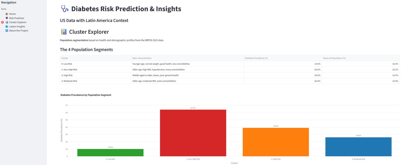
5.3. Profili dei Cluster e Interpretazione
Ho identificato 4 segmenti di popolazione distinti basati sulle loro caratteristiche di salute.
| Cluster | Numero di Persone | Caratteristiche Principali | Prevalenza Diabete (%) | Livello di Rischio | Raccomandazione |
|---|---|---|---|---|---|
| 0 | 95,187 | Giovani adulti, peso normale, buona salute generale, poche comorbidità | 10.0% | Basso Rischio | Prevenzione generale |
| 1 | 66,017 | Anziani, alto BMI, ipertensione, multiple comorbidità | 64.0% | Rischio Molto Alto | Screening prioritario e intervento intensivo |
| 2 | 37,846 | Mezza età fino ad anziani, obesi, cattiva salute auto-riferita | 39.0% | Alto Rischio | Programmi mirati sullo stile di vita |
| 3 | 62,539 | Anziani, BMI moderato, alcune comorbidità | 26.0% | Rischio Moderato | Educazione preventiva e monitoraggio regolare |
# 5.3 Cluster Profiles and Interpretation - Visualization
# Create a clean summary for plotting
viz_data = pd.DataFrame({
'Cluster Profile': [
'0: Low Risk (Young, healthy)',
'1: Very High Risk (Older, obese, comorbidities)',
'2: High Risk (Obese, poor health)',
'3: Moderate Risk (Older, moderate BMI)'
],
'Diabetes Prevalence (%)': [10.0, 64.0, 39.0, 26.0],
'Size (n)': [95187, 66017, 37846, 62539]
})
fig = px.bar(
viz_data,
x='Cluster Profile',
y='Diabetes Prevalence (%)',
text='Diabetes Prevalence (%)',
title='Diabetes Prevalence by Population Segment',
color='Cluster Profile',
color_discrete_sequence=['#2ca02c', '#d62728', '#ff7f0e', '#1f77b4']
)
fig.update_traces(texttemplate='%{text:.1f}%', textposition='outside')
fig.update_layout(
yaxis_title='Diabetes Prevalence (%)',
xaxis_title='Cluster Profile',
showlegend=False,
height=550
)
fig.show()
Insights Chiave:
- Cluster 1 è il gruppo a rischio più alto (64% prevalenza diabete). È composto principalmente da anziani con obesità, ipertensione e multiple comorbidità. Questo gruppo dovrebbe essere prioritizzato per screening aggressivo e intervento.
- Cluster 0 rappresenta il segmento più sano — principalmente giovani con buone abitudini di vita e basso rischio.
- Cluster 2 mostra che l’obesità combinata con cattiva salute auto-riferita aumenta significativamente il rischio, anche in mezza età.
- Età e BMI continuano a essere fattori dominanti nella segmentazione del rischio, rafforzando i risultati delle fasi di EDA e modellazione.
Questi cluster forniscono insights concreti per la politica di sanità pubblica in Argentina e America Latina. Ad esempio, le risorse potrebbero essere concentrate sul Cluster 1 ("Anziani Obesi ad Alto Rischio") attraverso programmi comunitari di screening e interventi sullo stile di vita.
6. Contesto Latam e Confronti
Per rendere l’analisi più rilevante per l’Argentina e l’America Latina, ho arricchito i risultati del BRFSS USA con dati regionali della PAHO e dell’Atlante del Diabete IDF.
6.1. Indicatori Chiave Latam (Sud e Centro America)
| Indicatore | Valore 2024 | Proiezione 2050 | Osservazione |
|---|---|---|---|
| Prevalenza standardizzata per età | 10.1% | 11.5% | Previsto aumento costante |
| Persone con diabete | 35.4 milioni | 51.5 milioni | +45% crescita prevista |
| Diabete non diagnosticato | ~30.4% | - | Elevato carico nascosto |
| Copertura del trattamento (Americhe, 30+ anni) | ~57–59% | - | Significativo gap di trattamento |
Fonte: Atlante del Diabete IDF & dati PAHO
6.2. Confronto: Dati USA vs Contesto Latam
- Nel dataset BRFSS 2023 degli USA, il tasso osservato di diabete è 14.62%.
- In Sud e Centro America, la prevalenza attuale è 10.1% (2024), ma si prevede che raggiunga 11.5% entro il 2050.
- Il cluster a rischio più alto (Cluster 1) mostra un tasso di diabete del 64% — molto più alto delle medie USA e Latam. Ciò suggerisce che individui con profili simili (età avanzata + obesità + comorbidità) rappresentano un gruppo critico ad alto rischio in tutta la regione.
- La forte influenza di BMI, età e comorbidità nel mio modello è coerente con i fattori di rischio noti in America Latina, dove l’aumento dell’obesità è un motore principale dell’epidemia di diabete.
6.3. Implicazioni per Argentina e America Latina
La combinazione dei risultati di clustering e dei dati regionali evidenzia la necessità di strategie di prevenzione mirate:
- Prioritizzare screening e interventi sullo stile di vita per anziani con obesità e ipertensione (simile al Cluster 1).
- Affrontare l’elevato tasso di non diagnosticati (~30%) tramite programmi comunitari.
- Concentrarsi su fattori di rischio modificabili (controllo BMI e attività fisica), che hanno mostrato forte potere predittivo nel modello.
Questi risultati supportano lo sviluppo di politiche di sanità pubblica localizzate in Argentina, dove la prevalenza del diabete continua ad aumentare.
7. Conclusioni e Raccomandazioni
7.1. Sintesi del Progetto
Questo progetto ha analizzato il rischio di diabete utilizzando il dataset CDC BRFSS 2023 (~261k record) combinato con contesto Latam da PAHO e IDF.
Il lavoro è progredito attraverso:
- Preparazione approfondita dei dati e uso avanzato di SQL con DuckDB
- EDA completo con visualizzazioni interattive
- Feature engineering informata dal dominio (punteggi di rischio, gruppi età+BMI, conteggio comorbidità, ecc.)
- Modellazione predittiva (classificazione binaria)
- Segmentazione della popolazione con clustering K-Means
7.2. Risultati Principali
- Predittori più forti: BMI, età, salute generale e comorbidità sono emersi come i fattori più importanti.
- La prevalenza del diabete aumenta significativamente con l’età, passando da 4.07% nei giovani adulti (18–44) a 21.31% negli anziani (75+).
- Il BMI è emerso come uno dei predittori più forti, con prevalenza che sale da 6.9% nel peso normale a 30.0% in Obesità Classe III.
- Clustering ha identificato quattro segmenti di rischio, con il gruppo a rischio più alto (anziani obesi con comorbidità) che mostra un tasso di diabete del 64%.
- Prestazioni del modello: L’approccio binario ha ottenuto risultati ragionevoli, con Regressione Logistica che ha fornito il miglior recall (75.61%).
- Contesto Latam: La prevalenza crescente in Sud e Centro America (10.1% nel 2024 → 11.5% previsto nel 2050) e l’elevato tasso di non diagnosticati (~30%) rendono questi risultati altamente rilevanti.
7.3. Raccomandazioni
Per le Autorità Sanitarie (Argentina & Latam):
- Prioritizzare screening mirati per Cluster 1 (anziani con obesità, ipertensione e multiple comorbidità).
- Implementare programmi di prevenzione precoce focalizzati su gestione del peso e attività fisica.
- Affrontare il gap di trattamento migliorando l’accesso alle cure nei gruppi a basso reddito.
- Utilizzare strumenti di stratificazione del rischio come quello sviluppato qui per ottimizzare risorse limitate.
Per gli Individui:
- Monitoraggio regolare di BMI, pressione arteriosa e salute generale per identificare precocemente il rischio.
- Cambiamenti nello stile di vita (più attività fisica e mantenimento del peso sano) hanno un impatto elevato.
7.4. Limitazioni e Lavori Futuri
- Il modello si basa su dati auto-riferiti, che possono contenere bias.
- Il pre-diabete rimane difficile da prevedere accuratamente con questo dataset.
- Miglioramenti futuri potrebbero includere valori di laboratorio (HbA1c, glicemia a digiuno), storia familiare o dati geografici più dettagliati.
Questo progetto dimostra competenze di analisi dei dati end-to-end — dalla preparazione intensiva in SQL alla modellazione e agli insights concreti di sanità pubblica.
8. Dashboard Streamlit
🚀 Dashboard Interattiva Live
Puoi esplorare la versione completamente interattiva di questo progetto qui:
🔗 Apri Diabetes Risk Analyzer →
Screenshot dall’App Live
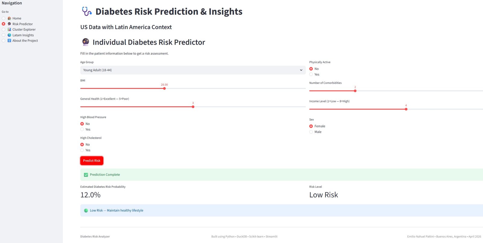
Cosa puoi fare nella dashboard live:
- Calcolare il tuo rischio personale di diabete usando il modello addestrato
- Esplorare i 4 segmenti di popolazione scoperti tramite clustering
- Visualizzare le tendenze del diabete e le proiezioni al 2050 per Sud e Centro America
Nota: La dashboard è distribuita su Streamlit Community Cloud ed è completamente interattiva.
Grazie per aver visto questo progetto!
Sentiti libero di contattarmi per domande o feedback.
# ======================================
# Export data for Streamlit Dashboard
# ======================================
# load the final table
con.execute("""
CREATE OR REPLACE TABLE diabetes_model_ready AS
SELECT * FROM diabetes_features
""")
# Export it to parquet
df_model_ready = con.execute("SELECT * FROM diabetes_model_ready").fetchdf()
# Save as parquet
df_model_ready.to_parquet("data/diabetes_model_ready.parquet", index=False)
print("✅ Successfully saved 'data/diabetes_model_ready.parquet'")
print(f"Shape: {df_model_ready.shape}")
print("Columns:", df_model_ready.columns.tolist())
✅ Successfully saved 'data/diabetes_model_ready.parquet' Shape: (261589, 29) Columns: ['diabetes_012', 'bmi', 'highbp', 'highchol', 'cholcheck', 'smoker', 'stroke', 'heartdiseaseorattack', 'physactivity', 'hvyalcoholconsump', 'genhlth', 'menthlth', 'physhlth', 'diffwalk', 'sex', 'agegroup', 'education', 'income', 'kidneydisease', 'asthma', 'copd', 'anyhealthcare', 'nodocbccost', 'age_group_cat', 'bmi_category', 'comorbidity_count', 'diabetes_risk_score', 'age_bmi_risk_group', 'lifestyle_score']
# ======================================
# Save the trained model for Streamlit
# ======================================
import joblib
import os
# Create the models folder if it doesn't exist
os.makedirs("models", exist_ok=True)
# Save the model
joblib.dump(model_lr, "models/logistic_regression_model.pkl")
print("✅ Model saved successfully as 'models/logistic_regression_model.pkl'")
print("Folder 'models' created if it didn't exist.")
✅ Model saved successfully as 'models/logistic_regression_model.pkl' Folder 'models' created if it didn't exist.
# Save the list of columns the model expects
import json
model_columns = list(X_train.columns)
with open("models/model_columns.json", "w") as f:
json.dump(model_columns, f)
print("✅ Model columns saved as 'models/model_columns.json'")
✅ Model columns saved as 'models/model_columns.json'